Build an AI-Powered Financial Digital Twin: Simulate a $100 Billion Bank with Python
- Build an AI-Powered Financial Digital Twin: Simulate a $100 Billion Bank with Python
- Introduction
- Step 1: Build a Synthetic Bank
- Step 2: Turn the Bank Into a Graph
- Step 3: Define Stress Scenarios
- Step 4: Start With Isolated Shocks
- Step 5: Simulate an Eight-Hour Cloud Failure
- Step 6: Connect Technology Failure to Customer Behavior
- Step 7: Calculate Financial Impact
- Step 8: Combine Multiple Risks
- Step 9: Stop Pretending One Scenario Is the Future
- Step 10: Turn the Twin Into a Decision Laboratory
- Step 11: Now Bring in the LLM
- Step 13: Visualize the Twin
- The Complete Workflow
- Running the Project
- Try It Yourself
- Real-World Applications
- Next Project: From Digital Twin to AI Risk Agent
- FAQ
Introduction
It is 9:00 AM.
One of your bank’s primary cloud regions suddenly becomes unavailable.
At first, this looks like a technology incident.
Engineers investigate the infrastructure. Applications attempt to fail over. Incident-response teams join calls.
But then something more interesting happens.
- Payment-processing capacity falls.
- Transactions begin piling up.
- Customers cannot complete payments.
- Some customers lose confidence and start moving money elsewhere.
- Deposit withdrawals increase.
- Liquidity begins falling.
What started as a cloud outage has become a financial risk event.
Now imagine you are sitting in the bank’s crisis-management room.
Executives start asking questions.
- How many customers are affected?
- How large could the payment backlog become?
- What happens to liquidity?
- Which applications are creating the largest blast radius?
- Would activating the backup region one hour earlier materially improve the outcome?
- And what happens if the cloud failure occurs at the same time as a market shock, deposit run, and counterparty default?
You cannot safely answer those questions by experimenting on a real bank.
So we are going to build another bank.
A virtual one.
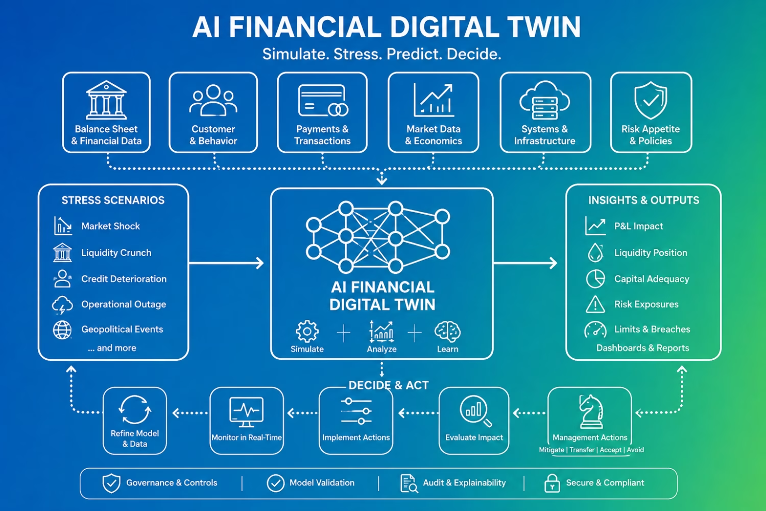
In this tutorial, we’ll explore an AI-powered Financial Digital Twin: a synthetic $100 billion bank that we can deliberately stress, break, recover, and analyze without touching real customers or real money.
The project combines graph modeling, discrete-event simulation, financial risk models, Monte Carlo simulation, management-action experiments, dashboards, and an optional LLM interpretation layer.
The complete source code is available in the AI Financial Digital Twin GitHub repository.
What You’ll Build
By the end of this tutorial, you’ll understand how to:
✔ Create a synthetic virtual bank
✔ Represent dependencies between infrastructure, applications, customers, and financial risks
✔ Model payment queues and recovery
✔ Propagate technology failures into business consequences
✔ Stress liquidity, credit, and market risk
✔ Run Monte Carlo simulations instead of trusting one scenario
✔ Test management interventions
✔ Use an LLM to explain validated simulation results
✔ Separate deterministic financial calculations from generative AI
Why This Problem Matters
Modern banks are complicated networks.
- A payment service depends on an application.
- That application depends on databases and cloud infrastructure.
- Customers depend on the payment service.
- Deposits depend on customer behavior.
- Liquidity depends partly on deposits.
- Capital can be affected by financial losses.
Yet organizations often analyze these risks separately.
The technology team asks:
“Are our systems available?”
The operations team asks:
“How many payments are delayed?”
Treasury asks:
“How much liquidity do we have?”
Risk management asks:
“Are any limits breached?”
Senior management ultimately needs a different answer:
How are all these things connected?
That is the problem a Financial Digital Twin attempts to explore.
The project creates a synthetic $100 billion bank containing balance-sheet information, customers, counterparties, applications, infrastructure, cloud environments, payment systems, and financial-risk relationships.
Instead of looking at one system at a time, we can ask:
If this component fails, what happens next?
Understanding a Digital Twin
The phrase digital twin sounds more complicated than it is.
Imagine building a flight simulator.
You don’t need to crash a real aircraft to study an engine failure.
Instead, the simulator contains a model of the aircraft.
You change something:
Engine fails.
The simulator calculates what happens next.
A Financial Digital Twin follows the same basic idea.
Instead of modeling an aircraft, we model a bank.
REAL BANK
   │
   │ simplified representation
   ▼
DIGITAL TWIN
   │
   ├── Customers
   ├── Deposits
   ├── Loans
   ├── Counterparties
   ├── Applications
   ├── Cloud infrastructure
   ├── Payment systems
   └── Risk limits
We can then inject hypothetical events.
Normal Bank
     ↓
Inject Stress
     ↓
Simulate Propagation
     ↓
Measure Consequences
     ↓
Test Response
That last step is particularly important.
A useful digital twin doesn’t only tell us:
“Something bad happened.”
It lets us ask:
“What would happen if we changed something?”
The Architecture
At a high level, this project looks like this:
Bank + Scenario + Risk Configuration
                │
                ▼
        Synthetic Bank State
          ┌─────┴─────┐
          ▼           ▼
   Dependency      Scenario
      Graph          Engine
                       │
        ┌──────────────┼──────────────┐
        ▼              ▼              ▼
     Market          Credit       Liquidity
     Engine           Engine        Engine
                       │
                       ▼
               Operational
                 Simulator
                       │
                       ▼
                  Risk KPIs
                       │
          ┌────────────┼────────────┐
          ▼            ▼            ▼
      Risk Limits   Monte Carlo   Actions
          │            │            │
          └────────────┼────────────┘
                       ▼
               Validated Results
                  ┌────┴────┐
                  ▼         ▼
             Dashboards    LLM
                         Explanation
The repository separates these responsibilities into modules for data generation, bank state, configuration, dependency graphs, scenario orchestration, market risk, credit risk, liquidity, operational simulation, metrics, Monte Carlo experiments, management actions, visualization, and AI explanation.
That modular design matters.
We do not want one giant notebook where every calculation depends on every other cell.
We want a system whose components have clear responsibilities.
Step 1: Build a Synthetic Bank
Before we can break our bank, we need one.
The project generates synthetic data representing a $100 billion institution.
Why synthetic data?
Because the purpose here is learning and experimentation.
Real banking data can contain confidential customer information, commercially sensitive exposures, security details, and regulatory constraints.
A synthetic environment lets us experiment safely.
Conceptually, our bank state contains things such as ( Refer the Github code for full details):
Bank
├── Balance Sheet
├── Customers
│   ├── Retail
│   ├── SME
│   ├── Corporate
│   └── Private Banking
├── Counterparties
├── Applications
├── Infrastructure
├── Cloud Regions
├── Payment Services
└── Risk Metrics
The important lesson isn’t the exact number of rows in a DataFrame.
It is the idea of state.
At any moment, our virtual bank has a state.
For example:
bank = create_synthetic_bank()Think of that object as a snapshot of our virtual world.
Then a scenario transforms that world.
Baseline State
      ↓
Stress Event
      ↓
Stressed State
This pattern appears everywhere in simulation engineering.
Step 2: Turn the Bank Into a Graph
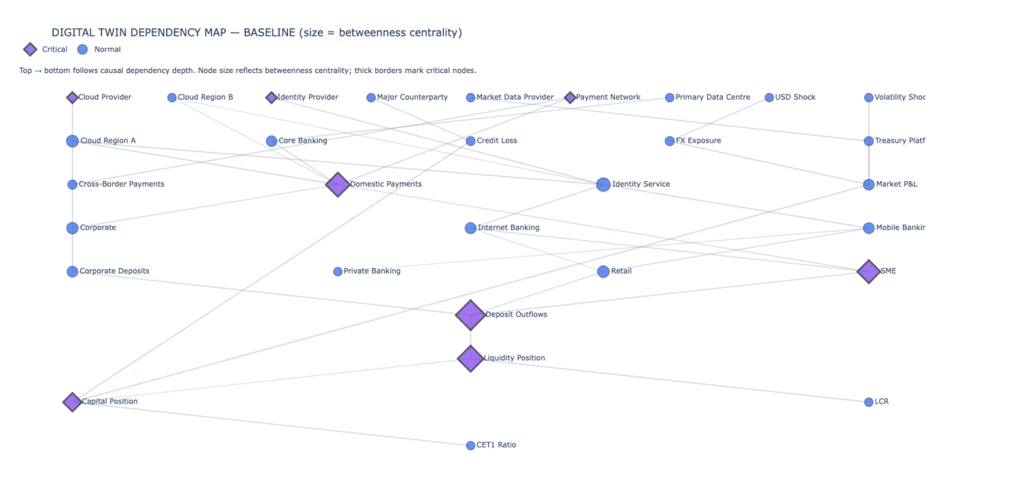
Here is where the project becomes much more interesting.
A spreadsheet can tell us which applications exist.
It cannot naturally tell us how failure spreads through them.
For that, we need a graph.
Understanding Graphs
A graph contains two things:
Nodes — things.
Edges — relationships between things.
Imagine:
Cloud Region A
      ↓
Payment App
      ↓
Payment Service
      ↓
Corporate Customers
      ↓
Deposits
      ↓
Liquidity
Each box is a node.
Each arrow represents a dependency.
The project uses a directed NetworkX graph to represent these relationships. It can identify downstream nodes, blast radius, critical nodes, high-betweenness nodes, single points of failure, cloud concentration, affected applications, customer segments, and financial-risk nodes.
You can think of the graph as the bank’s dependency map.
Suppose Cloud Region A fails.
We can ask:
affected = graph.descendants("Cloud Region A")Conceptually, we are saying:
Show me everything downstream that might depend on this component.
That changes the question from:
“Which server failed?”
to:
“What business consequences can this failure reach?”
Understanding Blast Radius
Imagine knocking over one domino.
If nothing depends on it, the damage stops there.
But if that domino is connected to 50 others, the consequences spread.
The blast radius describes how much of our system sits downstream of a failure.
                   Cloud A
                      │
              ┌───────┴───────┐
              ▼               ▼
        Payments App       CRM App
              │               │
              ▼               ▼
        Payment Service   Customer Service
              │
       ┌──────┴──────┐
       ▼             ▼
    Retail       Corporate
A highly connected component deserves attention even if the component itself looks small.
This is one reason graph analysis is useful for enterprise risk.
Risk is often hiding in the connections, not just the components.
Step 3: Define Stress Scenarios
Now we need something bad to happen.
Instead of hard-coding every scenario into Python, the project uses YAML configuration files.
That means we can describe a stress event separately from the engine that executes it.
The scenario library includes:
USD fall
Deposit run
Payment outage
Volatility shock
Cloud failure
Counterparty default
Eight-hour cloud-region failure
Combined stress
Why is configuration-driven simulation useful?
Because tomorrow’s experiment might be different.
Today:
Cloud backup activates after 3 hoursTomorrow:
Cloud backup activates after 1 hourWe shouldn’t have to redesign the simulation engine just to test that hypothesis.
This gives us a clean separation:
Scenario Definition
        ↓
Simulation Engine
        ↓
Results
Step 4: Start With Isolated Shocks
Before creating a giant financial crisis, the project runs individual scenarios.
This is good experimental design.
Suppose you mix six ingredients into a recipe and the food tastes terrible.
Which ingredient caused the problem?
You don’t know.
Simulation works the same way.
The project first evaluates six shocks independently: USD decline, deposit run, payment outage, volatility shock, cloud failure, and counterparty default. Each begins from the same synthetic baseline.
That lets us observe:
Baseline → Market Shock
Baseline → Deposit Shock
Baseline → Payment Shock
Baseline → Volatility Shock
Baseline → Cloud Shock
Baseline → Credit Shock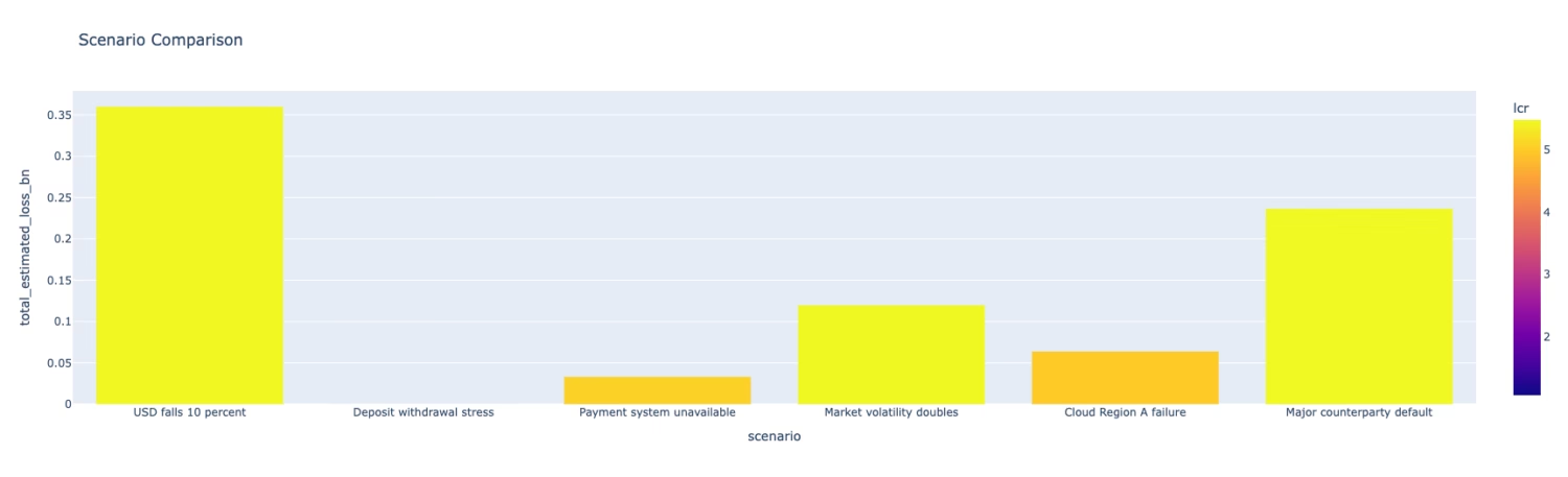
Only after understanding these pieces should we combine them.
This is a valuable habit for almost any AI or simulation project:
Start interpretable. Then add complexity.
Note, not all scenarios will trigger NetworkX and SImPy to navigate the bank graph. The bank graph created is primarily used only if the scenario covers a operational impact like cloud failure.
                ISOLATED SCENARIO
                       │
                       ▼
                ScenarioEngine
                       │
      ┌────────────────┼────────────────┐
      ▼                ▼                ▼
   Market           Credit         Operational
   Shock            Shock             Shock
      │                │                │
      ▼                ▼                ▼
Market Engine     Credit Engine     NetworkX
                                       │
                                       ▼
                                     SimPy
Step 5: Simulate an Eight-Hour Cloud Failure
Now we reach the project’s most intuitive experiment.
Imagine Cloud Region A disappears.
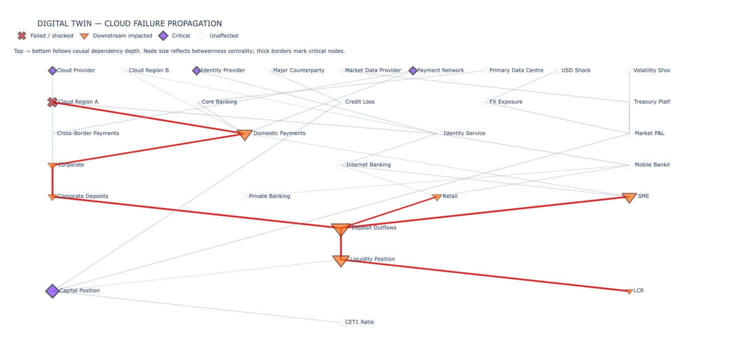
The configured timeline looks roughly like this:
Hour 0
Cloud Region A fails
      │
      ▼
Hours 0–3
Backup unavailable
      │
      ▼
Hour 3
Region B activates
      │
      ▼
Hours 3–8
70% processing capacity
      │
      ▼
Hour 8
Region A recovers
      │
      ▼
Temporary 125% capacity
      │
      ▼
Payment backlog clears
Those capacity assumptions come from the project’s configured scenario.
Notice something important.
Infrastructure recovery is not the same as business recovery.
Imagine a supermarket checkout system goes offline.
During the outage, 1,000 customers form a queue.
Then the computers restart.
Is the problem solved?
No.
You still have 1,000 customers waiting.
Bank payments behave similarly.
Infrastructure Restored
        ≠
Business Recovered
The project explicitly models the distinction between restoring processing capacity and clearing the accumulated payment backlog.
That is where SimPy enters the picture.
Understanding Discrete-Event Simulation
Suppose we want to model an airport.
Passengers arrive.
Security processes passengers.
Queues grow.
Additional lanes open.
Queues shrink.
We don’t need to calculate every millisecond.
We care about events.
That is discrete-event simulation.
In our bank:
Payments arrive
      ↓
Processing capacity handles payments
      ↓
Capacity falls
      ↓
Backlog grows
      ↓
Backup activates
      ↓
Capacity increases
      ↓
Backlog eventually clears
SimPy helps represent these time-dependent processes.
The operational simulator models payment arrivals, processing capacity, backlog, failover, and recovery.
This gives us something a static spreadsheet cannot:
time.
And time matters enormously during an outage.
Step 6: Connect Technology Failure to Customer Behavior
A digital twin becomes valuable when consequences cross domain boundaries.
Our cloud outage shouldn’t stop at:
Application unavailableWe want:
Cloud Failure
      ↓
Application Failure
      ↓
Payment Disruption
      ↓
Customer Impact
      ↓
Withdrawal Behavior
      ↓
Deposit Outflow
      ↓
Liquidity Consumption
The project’s dependency graph identifies the affected downstream components, while customer and financial models translate operational disruption into modeled consequences.
This is a form of causal propagation modeling.
Be careful with that phrase.
It does not mean the system has magically discovered real-world causality.
We explicitly created relationships and assumptions describing how effects propagate.
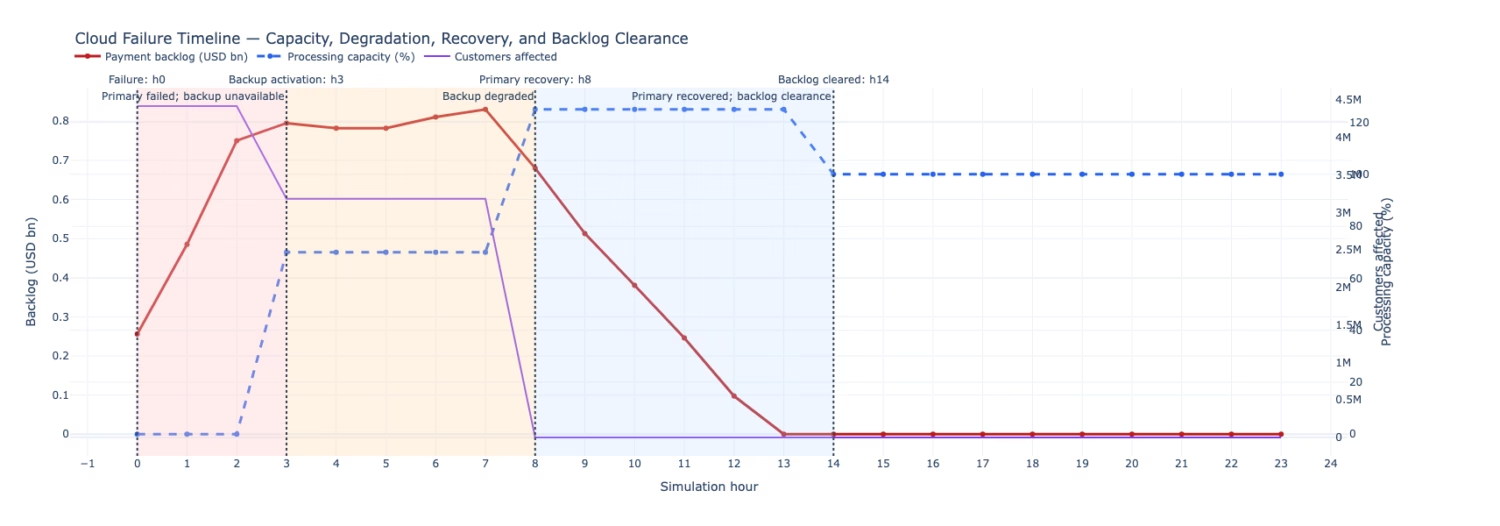
The simulation answers:
“Given these modeled relationships and assumptions, what happens?”
It does not prove:
“This is exactly what would happen in a real bank.”
That distinction is essential.
Step 7: Calculate Financial Impact
Now our operational event enters the financial world.
The project contains separate engines for market, credit, and liquidity impacts.
Think of them as specialized calculators.
Scenario
   │
   ├── Market Engine
   │      └── FX / volatility effects
   │
   ├── Credit Engine
   │      └── Expected/default losses
   │
   ├── Liquidity Engine
   │      └── Deposits / cash / HQLA
   │
   └── Operational Simulator
          └── Payments / outages / recovery
This architecture gives us another useful engineering principle:
Don’t ask an LLM to do calculations that deterministic software can perform more reliably.
We’ll return to that shortly.
Understanding Liquidity Risk
Liquidity is essentially the bank’s ability to meet its payment obligations when they come due.
Imagine you own a house worth $1 million.
But you have only $20 in your checking account.
Someone asks you to pay a $5,000 bill today.
You may be wealthy.
But you have a liquidity problem.
Banks face a much more complicated version of this problem.
If many depositors withdraw money quickly, available liquidity can become stressed.
The prototype calculates a simplified Liquidity Coverage Ratio conceptually as:
                High-Quality Liquid Assets
Prototype LCR = ──────────────────────────
                    Net Cash Outflows
But this deserves a large warning label.
The repository explicitly describes this as a simplified prototype metric, not a regulatory LCR implementation or determination of regulatory compliance.
That is exactly how we should present it.
Step 8: Combine Multiple Risks
Real crises rarely arrive politely, one at a time.
Imagine the bank experiences:
USD shock
       +
Market volatility
       +
Deposit withdrawals
       +
Counterparty default
       +
Cloud impairment
       +
Payment disruption
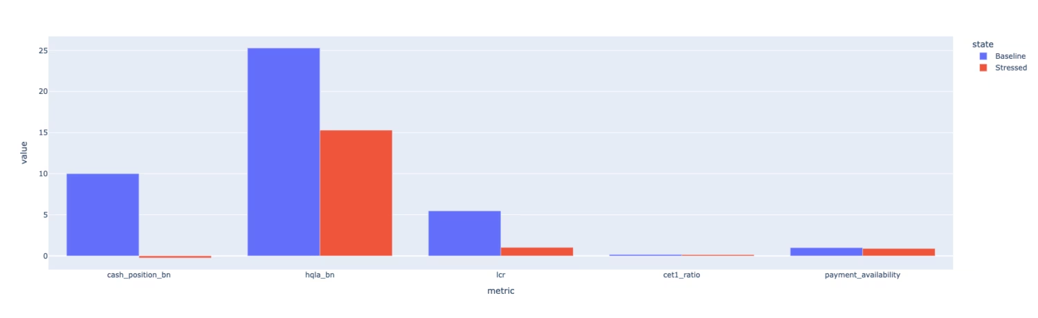
The project’s flagship combined_stress scenario does exactly this.
Its configured scenario includes a 10% USD shock, a 2× volatility multiplier, withdrawals across several customer segments, default of a synthetic counterparty, a credit probability-of-default multiplier, and cloud/payment impairment.
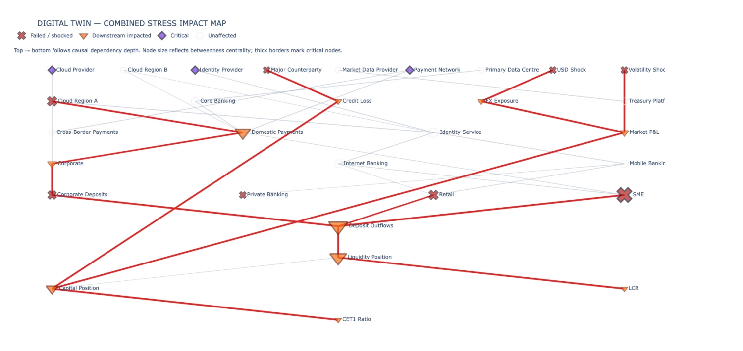
Crucially, the engine runs these conditions together.
It does not simply calculate:
Market loss
+ Credit loss
+ Liquidity loss
+ Operational loss
and call that a crisis.
Why?
Because systems interact.
A liquidity intervention might change available assets.
An operational intervention might change customer consequences.
One action can affect another risk domain.
Complex systems are rarely perfectly additive.
Step 9: Stop Pretending One Scenario Is the Future
So far we have been saying things like:
Withdrawal rate = X
Recovery time = Y
Market shock = Z
But reality doesn’t give us those values in advance.
Recovery might take four hours.
Or six.
Or nine.
Customers might withdraw more than expected.
Or less.
Market conditions might be milder or worse.
So instead of asking:
“What happens under one scenario?”
we ask:
“What happens across many plausible variations of this scenario?”
Welcome to Monte Carlo simulation.
Understanding Monte Carlo Simulation
Imagine a pair of dice.
You cannot confidently predict the next roll.
But you can roll them 10,000 times and understand the distribution of outcomes.
Monte Carlo simulation uses the same idea.
Instead of dice, we sample uncertain model inputs.
              Scenario
                 │
        ┌────────┼────────┐
        ▼        ▼        ▼
      Run 1    Run 2    Run 3  ... Run 1000
        │        │        │
        └────────┼────────┘
                 ▼
         Outcome Distribution
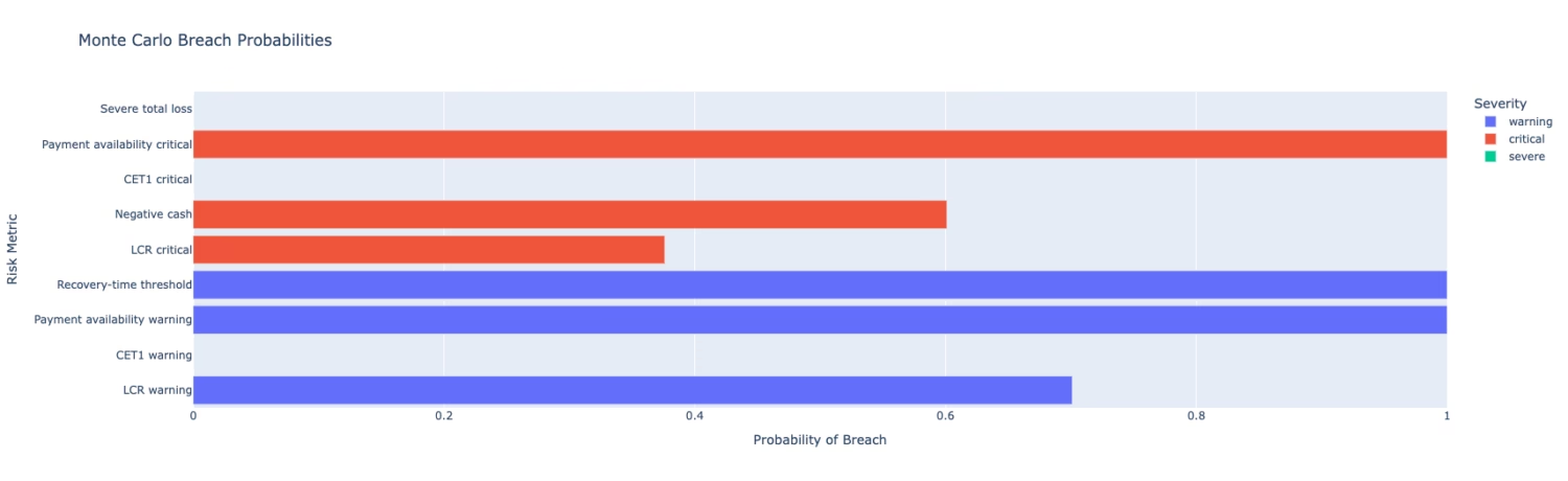
The project runs 1,000 stochastic variations of its combined stress scenario using random seed 42.
Variables sampled include factors such as the USD shock, volatility, withdrawal rates, recovery duration, and counterparty default-loss multiplier.
Instead of receiving one number, we can examine things like:
P5
Median
P95
Probability of limit breach
For example:
"What is the median modeled outcome?"

"What does a severe tail outcome look like?"

"How frequently is a configured limit breached?"
That is much more informative than presenting one deterministic result as destiny.
A Critical Monte Carlo Lesson
There is a trap here.
Suppose 80% of our simulations breach a liquidity threshold.
Can we say:
“There is an 80% chance the bank will breach its liquidity threshold.”
No.
The project’s documentation makes the same distinction: Monte Carlo frequencies are frequencies under the prototype’s configured assumptions, not calibrated estimates of real-world event probabilities.
This is one of the most important lessons in simulation.
A model tells you what happens inside its modeled world.
The quality of the conclusion depends on the quality of the assumptions.
Step 10: Turn the Twin Into a Decision Laboratory
Predicting bad outcomes is useful.
Testing possible responses is better.
Imagine management asks:
“What if we activate the backup region faster?”
We can rerun the cloud scenario with a different assumption.
Conceptually:
result = engine.run(
    "cloud_region_a_8hr",
    overrides={
        "operational": {
            "backup_activation_delay_hours": 1
        }
    }
)
Now we can compare:
3-Hour Backup Activation
           vs
1-Hour Backup Activation
and examine differences in payment backlog, customers affected, deposit outflow, operational loss, liquidity use, prototype LCR, and total recovery time.
This is where a digital twin becomes a decision laboratory.
Test Management Actions
The project goes further than changing one outage parameter.
Its management-action engine can simulate interventions such as:
- activating a backup region,
- prioritizing critical payments,
- selling liquid securities,
- drawing a liquidity facility,
- increasing an FX hedge,
- contacting high-risk corporate depositors.
The important architectural idea is that an action does not simply receive an invented score like:
"Activate backup = +20 resilience points"Instead, the action changes explicit simulation parameters.
Then the scenario runs again.
Conceptually:
Stress Scenario
      │
      ▼
   No Action
      │
      ▼
   Outcome A


Stress Scenario
      │
      ▼
Management Action
      │
      ▼
Rerun Simulation
      │
      ▼
   Outcome B
Then we compare A and B.
This is much more defensible than attaching arbitrary benefits to actions.
Why Combined Actions Must Be Simulated Together
Imagine management takes three actions.
It would be tempting to calculate:
Action A saves $10M
Action B saves $20M
Action C saves $15M

Total benefit = $45M
But what if A changes the conditions under which B operates?
Or B makes part of C unnecessary?
The project therefore runs combined interventions simultaneously instead of simply adding individual action benefits.
That illustrates an important systems principle:
Interactions matter.
Step 11: Now Bring in the LLM
We’ve reached the AI layer.
And this project makes an architectural decision that deserves attention.
The LLM is not the financial model.
Python performs the calculations.
Python determines the metrics.
Python evaluates thresholds.
Python generates the propagation paths.
Then validated results are passed to the language model.
Financial Models
      +
Simulation
      +
Graph Analysis
      +
Risk Limits
      │
      ▼
Validated Structured Results
      │
      ▼
     LLM
      │
      ▼
Executive Explanation
The repository explicitly prevents the LLM layer from being responsible for financial-impact calculations, severity classifications, graph dependencies, scenario assumptions, thresholds, or claims of regulatory validity.
This is an excellent enterprise GenAI pattern.
Understanding the LLM’s Role
Imagine hiring two employees.
One is an accountant.
One is a communications specialist.
Would you ask the communications specialist to invent the financial statements?
Probably not.
Instead:
Accountant
    ↓
Validated Numbers
    ↓
Communications Specialist
    ↓
Clear Explanation
The LLM plays the second role.
Its job is to turn structured results into something an executive can understand.
For example, Python might produce:
payment_availability: ...
liquidity_consumed: ...
customers_affected: ...
risk_severity: ...
recovery_time: ...
The LLM can translate that into:
The simulated outage caused a material operational disruption.
Payment capacity deteriorated before the backup region became
available, creating a backlog that persisted beyond infrastructure
restoration...
The words are generated.
The underlying numbers are not.
That boundary dramatically reduces the opportunity for hallucinated financial calculations.
Why This Is a Better Enterprise AI Pattern
Many beginner GenAI applications follow this architecture:
Raw Data
   ↓
LLM
   ↓
"Please figure everything out."
That can work for low-risk tasks.
It is uncomfortable for high-stakes financial calculations.
A stronger pattern is:
Deterministic Systems
        ↓
Validated Data
        ↓
LLM Interpretation
        ↓
Human Decision Maker
The LLM handles language.
Specialized models handle calculation.
Humans remain responsible for decisions.
This principle applies far beyond banking.
You could use the same architecture for:
Healthcare analytics
Supply-chain simulations
Cybersecurity risk
Insurance modeling
Manufacturing
Energy systems
Enterprise operations
Step 13: Visualize the Twin
Simulation produces a lot of numbers.
Humans aren’t particularly good at reading thousands of numbers.
So the project uses Plotly to create operational, risk, dependency, and executive visualizations.
Different visualizations answer different questions.
A dependency graph answers:
Where can the failure propagate?
A time-series chart answers:
When did the backlog peak?
A Monte Carlo distribution answers:
How uncertain is the outcome?
A management-action comparison answers:
Which simulated intervention changed the outcome?
A dashboard answers:
What should I investigate first?
Visualization isn’t decoration.
It is part of the reasoning interface.
The Complete Workflow
We can now see the entire project as one pipeline.
1. Generate Synthetic Bank
             ↓
2. Build Dependency Graph
             ↓
3. Load Stress Scenario
             ↓
4. Inject Shock
             ↓
5. Trace Blast Radius
             ↓
6. Simulate Operations Over Time
             ↓
7. Calculate Financial Consequences
             ↓
8. Evaluate Risk Limits
             ↓
9. Run Monte Carlo Variations
             ↓
10. Test Management Actions
             ↓
11. Visualize Results
             ↓
12. Build Validated Context
             ↓
13. Ask LLM to Explain
             ↓
14. Human Reviews Decision
Notice how late the LLM appears.
That is intentional.
Most of the intelligence of this system comes from how the problem is modeled, not from simply calling a language model.
Running the Project
The main notebook entry point is notebooks/master_runner.ipynb. in the Github Repo.
The repository supports running it in Google Colab or using your preferred local Python environment. The notebook orchestrates the underlying modules rather than containing a separate calculation model.
At a high level:
git clone <repository>
cd AI-Financial-Digital-Twin
Then install the project dependencies and run the master notebook.
The OpenAI integration is optional. If you only want to study the digital-twin simulation, you don’t need the LLM interpretation layer.
The project writes generated artifacts such as scenario comparisons, Monte Carlo results, propagation traces, management-action comparisons, and executive summaries into its output area. With identical code, configuration, and random seed, the generated results are designed to be reproducible.
Try It Yourself
Once you understand the default project, don’t stop there.
The best way to understand simulation is to break the assumptions.
Beginner
Change the backup activation delay.
Try:
3 hours → 2 hours → 1 hourObserve what happens to the payment backlog and recovery time.
Then modify one withdrawal assumption.
Ask:
Which KPI responds most strongly?
Intermediate
Create a new scenario:
Cloud outage
+
Corporate deposit run
Then compare it with the cloud-only scenario.
Next, change backup capacity:
50%
70%
90%
100%
Plot capacity against recovery time.
You are now performing sensitivity analysis.
Advanced
Extend the dependency graph.
Add another cloud provider.
Create applications with different failover strategies.
Introduce correlated Monte Carlo inputs instead of assuming every uncertain variable can be sampled independently.
Then build an action optimizer that searches combinations of management interventions subject to constraints and costs.
At that point, you are moving from:
simulation
toward:
decision optimization.
Real-World Applications
The underlying ideas extend well beyond this synthetic bank.
Banking: Operational resilience, liquidity stress, payment disruption, concentration risk, counterparty exposure, and crisis exercises.
Insurance: Model how catastrophes propagate through claims, reinsurance, liquidity, and operations.
Cloud infrastructure: Study dependency concentration and the business consequences of regional failures.
Supply chains: Trace how one supplier failure propagates into factories, inventory, customers, and revenue.
Cybersecurity: Connect compromised infrastructure to business services and financial consequences.
Healthcare: Model hospital capacity, staffing constraints, patient queues, and infrastructure failures.
Manufacturing: Connect equipment failures with production capacity, queues, delivery delays, and revenue.
Different industries.
Same underlying question:
If this fails, what happens next?
Next Project: From Digital Twin to AI Risk Agent
Our digital twin can already answer:
“What happens if this scenario occurs?”
But imagine giving it another capability.
Instead of manually choosing management actions, an AI agent could inspect the simulated crisis, propose several interventions, ask the deterministic twin to evaluate each one, compare residual risks and constraints, and return the evidence to a human decision-maker.
That architecture could look like:
Observe Crisis
      ↓
AI Agent Proposes Actions
      ↓
Digital Twin Simulates Each Action
      ↓
Risk Engine Validates Outcomes
      ↓
Agent Compares Alternatives
      ↓
Human Approves
Now the LLM still doesn’t control financial truth.
It uses the Digital Twin as a tool for reasoning.
That is where this architecture gets even more interesting.
FAQ
What is a Financial Digital Twin?
A Financial Digital Twin is a virtual representation of a financial system that can be used to simulate scenarios, dependencies, stresses, and responses without experimenting on the real system.
Is a Financial Digital Twin the same as an LLM?
No. An LLM generates or interprets language. A digital twin models the state and behavior of a system. An LLM can be one component of a larger digital-twin architecture.
Why use NetworkX in a digital twin?
NetworkX represents components as nodes and dependencies as edges, making it possible to analyze propagation paths, critical components, and blast radius.
Why use SimPy?
SimPy supports discrete-event simulation. It is useful when events, queues, capacity constraints, outages, and recovery happen over time.
What is Monte Carlo simulation?
Monte Carlo simulation repeatedly runs a model with sampled inputs to create a distribution of possible modeled outcomes instead of relying on one deterministic scenario.
Can this project predict a real bank failure?
No. The repository uses synthetic data and simplified, uncalibrated assumptions. Its outputs are educational prototype simulation results, not real-world forecasts.
Does the LLM calculate the financial results?
No. The project’s LLM layer is optional and is designed to interpret validated Python results rather than calculate financial impacts or change risk classifications.
Why simulate management actions?
It allows decision-makers to compare hypothetical interventions by changing model parameters and rerunning the simulation.
Can this architecture work outside banking?
Yes. The graph + simulation + deterministic models + uncertainty analysis + LLM explanation pattern can be adapted to areas such as supply chains, manufacturing, insurance, cybersecurity, healthcare, and infrastructure.
Is this a regulatory stress-testing model?
No. The repository explicitly identifies itself as a synthetic feasibility prototype rather than an approved or regulatory banking model.
Discover more from Debabrata Pruseth
Subscribe to get the latest posts sent to your email.